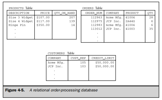
The relational model proposed by Dr. Codd was an attempt to simplify database structure. It eliminated the explicit parent/child structures from the database, and instead represented all data in the database as simple row/column tables of data values. Figure 4-5 shows a relational version of the network order-processing database in Figure 4-4.
Unfortunately, the practical definition of “What is a relational database?” became much less clear-cut than the precise, mathematical definition in Codd’s 1970 paper. Early relational database management systems failed to implement some key parts of Codd’s model. As the relational concept grew in popularity, many databases that were called “relational” in fact were not.
In response to the corruption of the term “relational,” Dr. Codd wrote an article in 1985 setting forth 12 rules to be followed by any database that called itself “truly relational.” Codd’s 12 rules have since been accepted as the definition of a truly relational DBMS. However, it’s easier to start with a more informal definition:
A relational database is a database where all data visible to the user is organized strictly as tables of data values, and where all database operations work on these tables.
The definition is intended specifically to rule out structures such as the embedded pointers of a hierarchical or network database. A relational DBMS can represent parent/child relationships, but they are represented strictly by the data values contained in the database tables.
1. The Sample Database
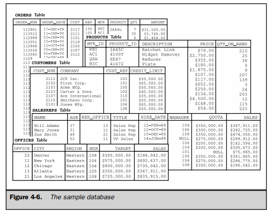
Figure 4-6 shows a small relational database for an order-processing application. This sample database is used throughout this book and provides the basis for most of the examples. Appendix A contains a complete description of the database structure and its contents.
The sample database contains five tables. Each table stores information about one particular kind of entity:
- The CUSTOMERS table stores data about each customer, such as the company name, credit limit, and the salesperson who calls on the customer.
- The SALESREPS table stores the employee number, name, age, year-to-date sales, and other data about each salesperson.
- The OFFICES table stores data about each of the five sales offices, including the city where the office is located, the sales region to which it belongs, and so on.
- The ORDERS table keeps track of every order placed by a customer, identifying the salesperson who took the order, the product ordered, the quantity and amount of the order, and so on. For simplicity, each order is for only one product.
- The PRODUCTS table stores data about each product available for sale, such as the manufacturer, product number, description, and price.
2. Tables
The organizing principle in a relational database is the table, a rectangular row/ column arrangement of data values. Each table in a database has a unique table name that identifies its contents. (Actually, each user can choose his or her own table names without worrying about the names chosen by other users, as explained in Chapter 5.)
The row/column structure of a table is shown more clearly in Figure 4-7, which is an enlarged view of the OFFICES table. Each horizontal row of the OFFICES table represents a single physical entity—a single sales office. Together the five rows of the table represent all five of the company’s sales offices. All of the data in a particular row of the table applies to the office represented by that row.
Each vertical column of the OFFICES table represents one item of data that is stored in the database for each office. For example, the CITY column holds the location of each office. The SALES column contains each office’s year-to-date sales total. The MGR column shows the employee number of the person who manages the office.
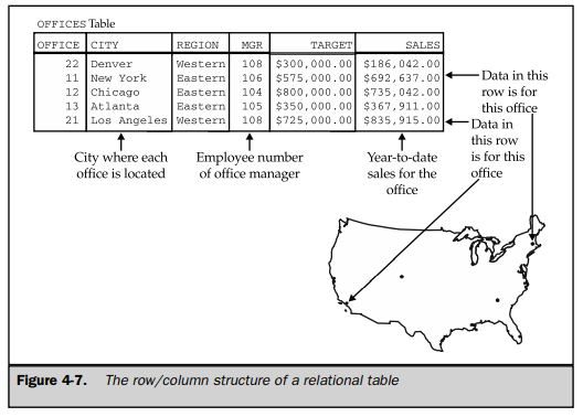
Each row of a table contains exactly one data value in each column. In the row representing the New York office, for example, the CITY column contains the value “New York”. The SALES column contains the value “$692,637.00”, which is the year- to-date sales total for the New York office.
For each column of a table, all of the data values in that column hold the same type of data. For example, all of the CITY column values are words, all of the SALES values are money amounts, and all of the MGR values are integers (representing employee numbers). The set of data values that a column can contain is called the domain of the column. The domain of the CITY column is the set of all names of cities. The domain of the SALES column is any money amount. The domain of the REGION column is just two data values, “Eastern” and “Western”, because those are the only two sales regions the company has.
Each column in a table has a column name, which is usually written as a heading at the top of the column. The columns of a table must all have different names, but there is no prohibition against two columns in two different tables having identical names. In fact, frequently used column names, such as NAME, ADDRESS, QTY, PRICE, and SALES, are often found in many different tables of a production database.
The columns of a table have a left-to-right order, which is defined when the table is first created. A table always has at least one column. The ANSI/ISO SQL standard does not specify a maximum number of columns in a table, but almost all commercial SQL products do impose a limit. Usually the limit is 255 columns per table or more.
Unlike the columns, the rows in a table do not have any particular order. In fact, if you use two consecutive database queries to display the contents of a table, there is no guarantee that the rows will be listed in the same order twice. Of course you can ask SQL to sort the rows before displaying them, but the sorted order has nothing to do with the actual arrangement of the rows within the table.
A table can have any number of rows. A table of zero rows is perfectly legal and is called an empty table (for obvious reasons). An empty table still has a structure, imposed by its columns; it simply contains no data. The ANSI/ISO standard does not limit the number of rows in a table, and many SQL products will allow a table to grow until it exhausts the available disk space on the computer. Other SQL products impose a maximum limit, but it is always a very generous one—two billion rows or more is common.
3. Primary Keys
Because the rows of a relational table are unordered, you cannot select a specific row by its position in the table. There is no “first row,” “last row,” or “thirteenth row” of a table. How, then, can you specify a particular row, such as the row for the Denver sales office?
In a well-designed relational database, every table has some column or combination of columns whose values uniquely identify each row in the table. This column (or columns) is called the primary key of the table. Look once again at the OFFICES table in Figure 4-7. At first glance, either the OFFICE column or the CITY column could serve as a primary key for the table. But if the company expands and opens two sales offices in the same city, the CITY column could no longer serve as the primary key. In practice, “ID numbers,” such as an office number (OFFICE in the OFFICES table), an employee number (EMPL_NUM in the SALESREPS table), and customer numbers (CUST_NUM in the CUSTOMERS table), are often chosen as primary keys. In the case of the ORDERS table, there is no choice—the only thing that uniquely identifies an order is its order number (ORDER_NUM).
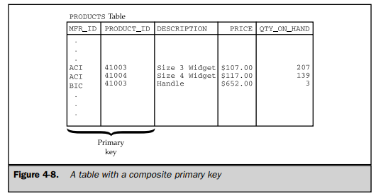
The PRODUCTS table, part of which is shown in Figure 4-8, is an example of a table where the primary key must be a combination of columns. The MFR_ID column identifies the manufacturer of each product in the table, and the PRODUCT_ID column specifies the manufacturer’s product number. The PRODUCT_ID column might make a good primary key, but there’s nothing to prevent two different manufacturers from using the same number for their products. Therefore, a combination of the MFR_ID and PRODUCT_ID columns must be used as the primary key of the PRODUCTS table. Every product in the table is guaranteed to have a unique combination of data values in these two columns.
The primary key has a different unique value for each row in a table, so no two rows of a table with a primary key are exact duplicates of one another. A table where every row is different from all other rows is called a relation in mathematical terms.
The name “relational database” comes from this term, because relations (tables with distinct rows) are at the heart of a relational database.
Although primary keys are an essential part of the relational data model, early relational database management systems (System/R, DB2, Oracle, and others) did not provide explicit support for primary keys. Database designers usually ensured that all of the tables in their databases had a primary key, but the DBMS itself did not provide a way to identify the primary key of a table. DB2 Version 2, introduced in April 1988, was the first of IBM’s commercial SQL products to support primary keys. The ANSI/ ISO standard was subsequently expanded to include a definition of primary key support, and today, most relational database management systems provide it.
4. Relationships
One of the major differences between the relational model and earlier data models is that explicit pointers, such as the parent/child relationships of a hierarchical database, are banned from relational databases. Yet obviously, these relationships exist in a relational database. For example, in the sample database, each salesperson is assigned to a particular sales office, so there is an obvious relationship between the rows of the OFFICES table and the rows of the SALESREPS table. Doesn’t the relational model “lose information” by banning these relationships from the database?
As shown in Figure 4-9, the answer to the question is “no.” The figure shows a close-up of a few rows of the OFFICES and SALESREPS tables. Note that the REP_ OFFICE column of the SALESREPS table contains the office number of the sales office where each salesperson works. The domain of this column (the set of legal values it may contain) is precisely the set of office numbers found in the OFFICE column of the OFFICES table. In fact, you can find the sales office where Mary Jones works by finding the value in Mary’s REP_OFFICE column (11) and finding the row of the OFFICES table that has a matching value in the OFFICE column (in the row for the New York office). Similarly, to find all the salespeople who work in New York, you could note the OFFICE value for the New York row (11) and then scan down the REP_OFFICE column of the SALESREPS table looking for matching values (in the rows for Mary Jones and Sam Clark).
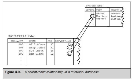
The parent/child relationship between a sales office and the people who work there isn’t lost by the relational model, it’s just not represented by an explicit pointer stored in the database. Instead, the relationship is represented by common data values stored in the two tables. All relationships in a relational database are represented this way. One of the main goals of the SQL language is to let you retrieve related data from the database by manipulating these relationships in a simple, straightforward way.
5. Foreign Keys
A column in one table whose value matches the primary key in some other table is called a foreign key. In Figure 4-9, the REP_OFFICE column is a foreign key for the OFFICES table. Although REP_OFFICE is a column in the SALESREPS table, the values that this column contains are office numbers. They match values in the OFFICE column, which is the primary key for the OFFICES table. Together, a primary key and a foreign key create a parent/child relationship between the tables that contain them, just like the parent/child relationships in a hierarchical database.
Just like a combination of columns can serve as the primary key of a table, a foreign key can also be a combination of columns. In fact, the foreign key will always be a compound (multicolumn) key when it references a table with a compound primary key. Obviously, the number of columns and the data types of the columns in the foreign key and the primary key must be identical to one another.
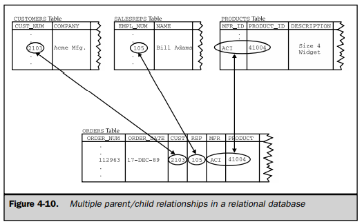
A table can contain more than one foreign key if it is related to more than one other table. Figure 4-10 shows the three foreign keys in the ORDERS table of the sample database:
- The CUST column is a foreign key for the CUSTOMERS table, relating each order to the customer who placed it.
- The REP column is a foreign key for the SALESREPS table, relating each order to the salesperson who took it.
- The MFR and PRODUCT columns together are a composite foreign key for the PRODUCTS table, relating each order to the product being ordered.
The multiple parent/child relationships created by the three foreign keys in the ORDERS table may seem familiar to you, and they should. They are precisely the same relationships as those in the network database of Figure 4-4. As the example shows, the relational data model has all of the power of the network model to express complex relationships.
Foreign keys are a fundamental part of the relational model because they create relationships among tables in the database. Unfortunately, like with primary keys, foreign key support was missing from early relational database management systems. They were added to DB2 Version 2, have since been added to the ANSI/ISO standard, and now appear in many commercial products.
Source: Liang Y. Daniel (2013), Introduction to programming with SQL, Pearson; 3rd edition.