The reason people use computers is different depending on the point in history in which one looks, but the military always seems to be involved. There have been many calculating devices built and used throughout history, but the first one that would have been programmable was designed by Charles Babbage. The military, as well as the mathematicians of the day, were interested in more accurate mathematical tables, such as those for logarithms. At the time, these were calculated by hand, but the idea that a machine could be built to compute more digits of accuracy was appealing. This would have been a mechanical device of gears and shafts, but it was not completed due to budget and contracting issues.
Babbage continued his work in design and created, on paper, a programmable mechanical device called the analytical engine in 1837. What does programmable mean? A calculation device is manipulated by the operator to perform a sequence of operations:
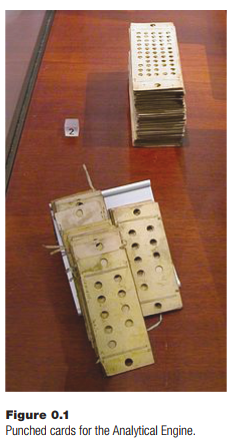
add this to that, then subtract this and divide by something else. On a modern calculator, this would be done using a sequence of key presses, but on older devices, it may involve moving beads along wires or rotating gears along shafts. Now imagine that the sequence of key presses can be encoded on some other media: a set of cams, or plugs into sockets, or holes punched into cards. This is a program.
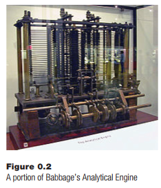
Such a set of punched cards or cams would be similar to a set of instructions written in English and given to a human to calculate, but would instead be coded in a form (language) that the computing device could use immediately. The direc- tions on the cards could be changed so that something new could be computed as needed. The difference engine only found logarithms and trigonometric functions, but a device that could be programmed in this way could, in theory, calculate anything. The analytical engine was programmed by punching holes in stiff cards, an idea that was derived from the Jacquard loom of the day. The location of holes indicated either an operation (e.g., add or subtract) or data (a number). A sequence of such cards was executed one at a time and yielded a value at the end.
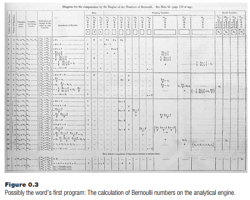
Although the analytical engine was never completed, a program was written for it, but not by Babbage. The world’s first programmer may have been a woman, Augusta Ada King, Countess of Lovelace. She worked with Babbage for a few years and wrote a program to compute Bernoulli numbers. This was the first algorithm ever designed for a computer and is often claimed to be the first computer program ever written, although it was never executed.
The concept of programmability is a more important development than is the development of analytical engines. The idea that a machine can be made to do different things depending on a user-defined set of instructions is the basis of all modern computers, while the use of mechanical calculation has become obsolete; it is too slow, expensive, and cumbersome. This is where it began, though, and the concept of programming is the same today.
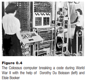
During World War II, computers were run using electricity. Work on breaking codes and building the atomic bomb required large amounts of computing. Initially, some of this was provided by rooms full of humans operating mechanical calculators, but they could not keep up with the demand, so electronic computers were designed and built. The first was Colossus, de- signed and built by Tommy Flowers in 1943. It was created to help break German military codes, and an updated version (Mark II) was built in 1944.
In the United States, there was a need for computational power in Los Alamos when the first nuclear weapons were being built. Electro-mechanical calculators were replaced by IBM punched-card calculators, originally designed for accounting. These were only a little faster than the humans using calculators, but could run twenty-four hours a day and made fewer errors. The punch- card computer was programmed by plugging wires into sockets to create new connections between components.
1. Numbers
The electronic computers described so far, and those of the 1940s generally, had almost no storage for numbers. Input was through devices like cards, and they had numbers on them. They were transferred to the computation unit, then moved ahead or back, and perhaps read again. Memory was a primitive thing, and various methods were devised to store just a few digits. A significant advance came when engineers decided to use binary numbers.
Electronic devices use current and voltage to represent information, such as sounds or pictures (radio and television). One of the simplest devices is a switch, which can open and close a circuit and turn things like lights on and off. Electricity needs a complete circuit or route from the source of electrons, the negative pole of a battery perhaps, to the sink, which could be the positive pole. Electrons, which is what electricity is, in a simple sense, flow from the negative to the positive poles of a battery. Electricity can be made to do work by putting devices in the way of the flow of electrons. Putting a lamp in the circuit can cause the lamp to light up, for example.
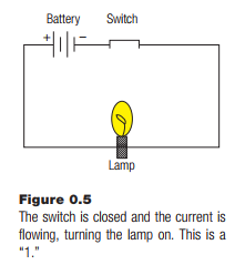
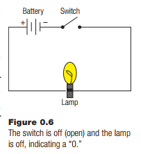
A switch makes a break in the circuit, which stops the electrons from flowing; they cannot jump the gap. This causes the lamp to go dark. This seems obvious to anyone with electric lights in their house, but what may not be so obvious is that this creates two states of the circuit, on and off. These states can be assigned numbers. Off is 0, for example, and on is 1. This is how most computers represent numbers: as on/off or 1/0 states. Let’s consider this in regards to the usual way we represent numbers, which is called positional numbering.
Most human societies now use a system with ten digits: 0, 1, 2, 3, 4, 5, 6, 7, 8, and 9. The number 123 is a combination of digits and powers of ten. It is a shorthand notation for 100 + 20 + 3, or 1 X 10² + 2*101 + 3*100. Each digit is multiplied by a power of ten and summed to get the value of the number. Anyone who has been to school accepts this and does not think about the value used as the basis of the system: ten. It simply happens to be the number of digits humans have on their hands. Any base would work almost as well.
Example: Base 4
Numbers that use 4 as a base can only have the digits 0, 1, 2, and 3. Each position in the number represents a power of 4. Thus, the number 123 is, in base 4, 1 X 42 + 2*41 + 3*40, which is 1 X 16 + 2*4 + 3 = 16 + 8 + 3 = 27 in traditional base 10 representation.
This could get confusing, what with various bases and such, so the numbers here are considered to be in base 10 unless specifically indicated otherwise by a suffix. For example, 1234 is 123 in base 4, whereas 1238 is 123 in base 8.
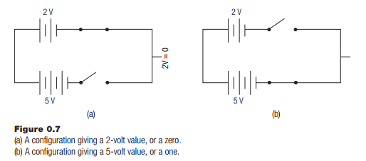
Binary numbers can have digits that are 1 or 0. The numbers are in base 2, and can therefore only have the digits 0 and 1. These numbers can be represented by the on/off state of a switch or transistor, an electronic switch, which why they are used in electronic computers. Modern computers represent all data as binary numbers because it is easy to represent those numbers in electronic form; a voltage is arbitrarily assigned to “0” and to “1.” When a device detects a particular voltage, it can then be converted into a digit, and vice-versa. If 2 volts is assigned to a 0, and 5 volts is assigned to a 1, then the circuit shown in Figure 0.7 could signal a 0 or 1, depending on what switch was selected.
Convert Binary Numbers to Decimal
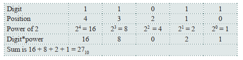
Consider the binary number 110112. The subscript “2” here means “base 2.” It can be converted into base 10 by multiplying each digit by its corresponding power of two and then summing the results.
Some observations:
- Terminology: A digit in a binary number is called a bit (for binary digit)
- Any even number has 0 as the low digit, which means that odd numbers have 1 as the low digit.
- Any exact power of two, such as 16, 32, 64, and so on, will have exactly one digit that is a 1, and all others will be 0.
- Terminology: A binary digit or bit that is 1 is said to be A bit that is 0 is said to be clear.
Convert Decimal Numbers to Binary
Going from base 10 to base 2 is more complicated than the reverse. There are a few ways to do the calculation, but here’s one that many people find easy to understand. If the lowest digit (rightmost) is 1, then the number is odd, and otherwise it is even. If the number 7310 is converted into binary, the rightmost digit is 1, because the number is odd.
The next step is to divide the number by 2, eliminating the rightmost binary digit, the one that was just identified, from the number. 7310/210 = 3610, and there can be no fractional part so any such part is to be discarded. Now the problem is to convert = 3610 to binary and then append the part already converted to that. Is 3610 even or odd? It is even, so the next digit is 0. The final two digits of 7310 in binary are 01.
The process is repeated:
Divide 36 by 2 to get 18, which is even, so the next digit is 0.
Divide 18 by 2 to get 9, which is odd, so the next digit is 1.
Divide 9 by 2 to get 4, which is even, so the next digit is 0.
Divide 4 by 2 to get 2, which is even, so the next digit is 0.
Divide 2 by 2 to get 1, which is odd, so the next digit is 1.
Divide 1 by 2 to get 0. When the number becomes 0, the process is complete.
The conversion process gives the binary numbers in reverse order (right to left) so the result is that 7310 = 10010012.
Is this correct? Convert this binary number into decimal again:
100 1 0012 = 1 X 20 + 1*23 + 1*26 = 1 + 8 + 64 = 7310.
A summary of the process for converting x into binary for is as follows:
Start at digit n=0 (rightmost)
repeat
If x is even, the current digit n is 0 otherwise it is 1.
Divide x by 2
Add 1 to n
If x is zero then end the repetition
Arithmetic in Binary
Computers do all operations on data as binary numbers, so when two numbers are added, for example, the calculation is performed in base 2. Base 2 is easier than base 10 for some things, and adding is one of those things. It’s done
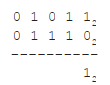
in the same way as in base 10, but there are only 2 digits, and twos are carried instead of tens. For example, let’s add 010112 to 011102:
![]()
Starting the sum on the right as usual, there is a 0 added to a 1 and the sum is 1, just as in base 10.
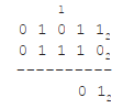
The next column in the sum contains two 1s. 1 + 1 is two, but in binary that is represented as 102. So, the result of 1+1 is 0 with a carry of 1 is as follows:
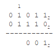
The next column has 1 + 0, but there is a carry of 1 so it is 1 + 0 + 1. That’s 0 with a 1 carried again:
Now the column is 1 + 1 with a 1 carried, or 1 + 1 + 1. This is 1 with a carry of 1:
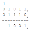
Finally, the leading digits are 0+0 with a carry of 1, or 0 + 0 + 1. The answer is 110012. Is this correct? Well, 010112 is 1110 and 011102 is 142, and 1110 + 1410=2510. The answer 110012 is, in fact, 2510.
Binary numbers can be subjected to the same operations as any other form of number (i.e., multiplication, subtraction, division). In addition, these operations can be performed by electronic circuits operating on voltages that represent the digits 1 and 0.
2. Memory
Adding memory to computers was another important advancement. A computer memory must hold steady a collection of voltages that represent digits, and the digits are collected into sets, each of which is a number. A switch can hold a binary digit, but switches are activated by people. Computer memory must store and recall (retrieve) numbers when they are required by a calculation without human intervention.
The first memories were rather odd things: acoustic delay lines stored numbers as a sound passing through mercury in a tube. The speed of sound allows a small number of digits, around 500, to be stored in transit from a speaker on one end to a receiver on the other. A phosphor screen can be built that is activated by an electric pulse and draws a bright spot on a screen that needs no power to maintain it. Numbers can be saved as bright and dark spots (1 and 0) and retrieved using light sensitive devices.
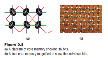
Other devices were used in the early years, such as relays and vacuum tubes, but in 1947 the magnetic core memory was patented, in which bits were stored as magnetic fields in small donut-shaped elements. This kind of memory was faster and more reliable than anything used before, and even held the data in memory without power being applied, a handy thing in a power failure. It was also expensive, of course.
This kind of memory is almost never used anymore, but its legacy remains in the terminology: memory is still frequently referred to as core, and a core dump is still what many people call a listing of the contents of a computer memory.
Current computers use transistors to store bits and solid state memories that can hold billions of bits (Gigabits), but the way they are used in the computer is still the same as it was. Bits are collected into groups of 8 (a byte) and then groups of multiple bytes to for a word. Words are collected into a linear sequence, each numbered starting at 0. These numbers are called addresses, and each word, and sometimes each byte, can be accessed by specifying the address of the data that is wanted. Acquiring the data element at a particular location is called a fetch, and placing a number into a particular location is a store. A computer program to add two numbers might be specified as follows:
- Fetch the number at location 21.
- Fetch the number at location 433.
- Add those two numbers.
- Store the result in location 22.
This may seem like a verbose way to add two numbers, but remember that this can be accomplished in a tiny fraction of a second.
Memory is often presented to beginning programmers as a collection of mailboxes. The address is a number identifying the mailbox, which also contains a number. There is some special memory in the computer that has no specific address, and is referred to in various ways. When a fetch is performed there is a question concerning where the value that was fetched goes. It can go to another memory location, which is a move operation, or it can go into one of these special locations, called registers.
A computer can have many registers or very few, but they are very fast memory units that are used to keep intermediate results of computations. The simple program above would normally have to be modified to give registers that are involved in the operations:
- Fetch the number at location 21 into register R0.
- Fetch the number at location 433 into register R1.
- Add R1 and R0 and put the result into R3.
- Store R3 (the result) in location 22.
This is still verbose, but more correct.
3. Stored Programs
The final critical step in creating the modern computer occurred in 1936 with Alan Turing’s theoretical paper on the subject, but an actual computer to employ the concept was not built until 1948 when the Manchester Small-Scale Experimental Machine ran what is considered to be the first stored program. It has been the basic method by which computers operate ever since.
The idea is to store a computer program in memory locations instead of on cards or in some other way. Programs and data now co-exist in memory, and this also means that computer programs have to be encoded as numbers; everything in a computer is a number. There are many different ways to do this, and many possible different instruction sets that have been implemented and various different configurations of registers, memory, and instructions. The computer hardware always does the same basic thing: first, it fetches the next instruction to be executed, and then it decodes it and executes it.
Executing an instruction could involve more accesses to memory or registers.
This repeated fetch then executes a process called the fetch-execute cycle, which is at the heart of all computers. The location or
address of the next instruction resides in a register called the program counter, and this register is incremented every time an instruction is executed, meaning that instructions will be placed in consecutive memory locations and will be fetched and executed naturally in that order. Sometimes the instruction is fetched into a special register too, called the instruction register, so that it can be examined quickly for important components like data values or addresses. Finally, a computer will need at least one register to store data; this is called the accumulator.
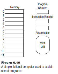
The stored program concept is difficult to understand. Imagine a computer that has 12-bit words as memory locations and that possesses the registers described above. This is a fictional machine, but it has some of the properties of an old computer from the 1960s called the PDP/8.
To demonstrate the execution of a program on a stored program computer, let’s use a very simple program: add 21 and 433, and place the answer in location 11. As an initial assumption, assume that the value 21 is in location 9 and 433 is in location 10. The program itself resides in consecutive memory locations beginning at address 0.
Note that this example is very much like the previous two examples, but in this case, there is only one register to put data into, the accumulator. The program could perhaps look like this:
- Fetch the contents of memory location 9 into the accumulator.
- Add the contents of memory location 10 to the accumulator.
- Store the contents of the accumulator into memory location 11.
The program is now complete, and the result 21 + 433 is in location 11. Computer programs are normally expressed in terms that the computer can immediately use, normally as terse and precise commands. The next stage in the development of this program is to use a symbolic form of the actual instructions that the computer will use.
The first step is to move the contents of location 9 to the accumulator. The instruction that does this kind of thing is called Load Accumulator, shorted as the mnemonic LDA. The instruction is in location 0:
0: LDA 9 # Load accumulator with location 9
The text following the character is ignored by the computer, and is really a comment to remind the programmer what is happening. The next instruction is to add the contents of location 10 to the accumulator; the instruction is ADD and it is placed in address 1:
1: ADD 10 # Add contents of address 10 to the accumulator
The result in the accumulator register is saved into the memory location at
address 11. This is a Store instruction:
2: STO 11 # Answer into location 11
The program is complete. There is a Halt instruction:
3: HLT # End of program</NL>
If this program starts executing at address 0, and if the correct data is in the correct locations, then the result 454 should be in location 11. But these instructions are not yet in a form the computer can use. They are characters, text that a human can read. In a stored program computer, these instructions must be encoded as numbers, and those numbers must agree with the ones the computer was built to implement.
An instruction must be a binary number, so all of the possible instructions have numeric codes. An instruction can also contain a memory address; the LDA instruction specifies a memory location from which to load the accumulator. Both the instruction
code and the address have to be placed into one computer word. The designers of the computer decide how that is done.
This computer has 12-bit words. Imagine that the upper 3 bits indicate what the instruction is. That is, a typical instruction is formatted as shown in Figure 0.12.
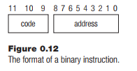
There are 9 bits at the lower (right) end of the instruction for an address, and 3 at the top end for the code that represents the instruction. The code for LDA is 3; the code for ADD is 5, and the code for STO is 6. The HLT on most computers is code 0. Here is what the program looks like as numbers:
Code 3 Address 9
Code 5 Address 10
Code 6 Address 11
Code 0 Address 0
These have to be made into binary numbers to be stored in memory. For the LDA instruction, the code 310 is 0112 and the address is 910 = 0000010012, so the instruction as a binary number is 011 0000010012, where the space between the code and the address is only present to make it obvious to a person reading it.
The ADD instruction has code 510, which is 1012, and the address is 10, which in binary is 000 1 0 1 02. The instruction is 10 1 00 0 00 1 0 1 02.
The STO instruction has code 6, which is 1102 and the address is 11, which is 0010112. The instruction is 110 0000010112.
The HLT instruction is code 0, or in 12-bit binary, 000 0000000002.
The codes are made up by the designers of the computer. Figure 0.13 shows an example of when memory is set up to contain this program.
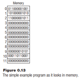
This is how memory looks when the program begins. The act of setting up the memory like this so that the program can execute is called loading. The binary numbers in memory locations 9 and 10 are 21 and 433, respectively, which are the numbers to be summed.
Of course, there are more instructions than these in a useful computer. There is not always a subtract instruction, but subtraction can be done by making a number negative and then adding, so there is often a NEGate instruction. Setting the accumulator to zero is a common thing to do so there is a CLA (Clear Accumulator) instruction; and there are many more.
The fetch-execute cycle involves fetching the memory location addressed by the program counter into the instruction register, incrementing the program counter, and then executing the instruction. Execution involves figuring out what instruction is represented by the code and then sending the address or data through the correct electronic circuits.
A very important instruction that this program does not use is a branch. The instruction BRA 0 causes the next instruction to be executed starting at memory location 0. This allows a program to skip over some instructions or to repeat some many times. A conditional branch changes the current instruction if a certain condition is true. An example would be “Branch if Accumulator is Zero (BAZ).” which is only performed if, as the instruction indicates, there is a value of zero in the accumulator. The combination of arithmetic and control instructions makes it possible for a programmer to describe a calculation to be performed very precisely.
Source: Parker James R. (2021), Python: An Introduction to Programming, Mercury Learning and Information; Second edition.